How AI Learns, part 1

What does it mean to say that an AI “learned” to do something? This article will be the part 1 of a series attempting to answer that question using as little math as possible. In this article, I will lay out the fundamental concepts of AI and machine learning, first by describing them in words and then by working through a couple of simple statistical examples. If you take one thing away from this article, make it this: machine learning, which is behind all modern AI, is just statistical modeling of data.

AI, short for “artificial intelligence”¹, refers to computer programs which can perform tasks requiring some degree of abstract reasoning. This is a broad class of programs, ranging from simple game-playing algorithms to ChatGPT, but does not include straighforward math problems, which were the first use for computers and still what they do at a low level. The challenge of AI is to express higher-level questions like “what object is in this picture” in the language of math and logic, that is, turn them into math problems, and then use algorithms to solve the math problems. Expressing questions in terms of math is fairly straighforward; the hard part is figuring out the algorithm, which is a series of calculations and rules for when to calculate what. But AI always consists of an algorithm that takes input and computes an output through a series of calculations, in order to answer some question that is baked into the AI by design.

There are two ways to find an algorithm for solving a problem: using learning, or not. We will address the “not” first. The earliest AI approaches, from before the 1970s or so, didn’t use learning to find algorithms. Instead, algorithms were worked out by hand and then hard-coded into the computer. This actually works for a lot of problems, such as playing board games. Eventually, scientists began working on algorithms to process languge. It was assumed that, because language follows grammatical rules, these rules could also be hard-coded into a program. But this failed, because the grammatical rules of most languages are far too complicated to write down. A better approach was needed.

The solution was to, in essence, let the computer figure the rules out by itself. Instead of explicitly coding in rules for an algorithm, machine learning defines a function with many adjustable parameters, called the model, which is also a type of algorithm. The model parameters function like knobs to adjust the output of the model. When using machine learning, we have training data, which consists of inputs and their correct outputs. The goal is to “learn” by adjusting the model parameters so the output, called the prediction, for a training input is as close to the correct output as possible. The reason this was such an important step forward is that numerous statistical methods already exist for predicting quantities from data. Thus the problem of finding rules to solve a problem reduces to statistical modeling of the inputs and outputs and their relationship.

This all sounds complicated, and it is. But you might already be familiar with an example of machine learning, in finding the line of best fit. This is called linear regression, and it is one of the simplest forms of machine learning. The figure below shows some data points and their line of best fit.

Left: A scatter plot of 30 projectile masses vs. their distance traveled when shot out of a cannon.
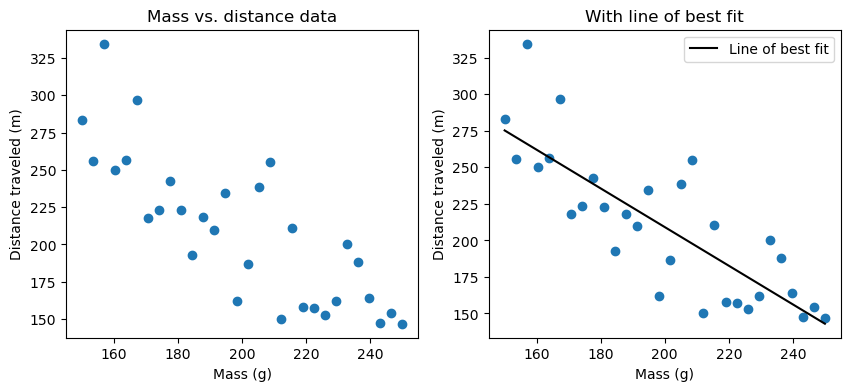
Right: Same data points, plus the line of best fit.

The line of best fit is an equation to predict values of our y-variable, written as $\hat{y}$ to show that it is predicted, for any value of our x-variable. We construct this line based on a set of data points $(x,y)$, trying to make it best predict the actual value of each $y$ in data from its corresponding $x$ (in other words, have the least error). The assumption here is that future values of $y$ will follow the same pattern as the data we already observed, and that’s why machine learning works in the first place.
The line of best fit is a function of the form $\hat{y}=mx + b$, where $m$ is the slope of the line and $b$ is the y-intercept (where the line crosses the y-axis, i.e., the value of $\hat{y}$ when $x=0$). $m$ and $b$ are the values that make the error in the model the smallest. What’s the error? In this case, it’s the average of the square of the vertical distance from each point to the line at the same $x$. In other words, it is $(\hat{y}-y)^2$ averaged over all data points, called the mean squared error or MSE.

The example below shows 30 data points showing the mass of a projectile vs. its distance traveled when shot out of a cannon. You can adjust the sliders to vary $m$ and $b$; read on once you think you’ve found the line of best fit.

With enough data points, the line of best fit would be $\hat{y}=-1.2x+450$, because that’s what I used to generate the data. But the line of best fit for these particular 30 points is something like $\hat{y}=-1.3x+470$, which is close but not exactly the same, because there are random fluctuations in distance traveled due to shape, air resistance, etc. I want to be clear that these are not measurement errors; those are small compared to the size of these deviations from the theoretical linear model. These are variations caused by factors other than mass, which we are just not considering in our model because they aren’t as important.

So if the distance traveled by a projectile clearly has a linear relationship with mass, but is not exactly defined by a function $y=mx+b$, how can we approximate $m$ and $b$ in order to get close? In short, probability.

First, let’s talk about what a probability distribution is. It is a function $p(x)$ that describes something observable and tells us how likely it is to observe a value of $x$ relative to all other possible values. We assume that our data is sampled² from an underlying probability distribution. The goal of machine learning is to learn (or “fit” or “train”) a model $p(x)$ from data so it best approximates the actual probability distribution of the data.

Let’s look at an example. Suppose we have 500 data points, where each represents the height in centimeters of a certain adult male. We want to model the distribution $p(x)$, where $x$ is a height in centimeters. Shown below is a histogram of 500 randomly-sampled heights. Each bar’s width is a range of x-values, and its height is the fraction of our data points that fall into that range. With enough data points, we should be able to assume that that fraction, the density, is the probability of a man’s height being in that range.

Male heights are known to follow a normal, or Gaussian, distribution. This is a function of $x$ that has two parameters, $\mu$ and $\sigma$, so we can write $p(x)$ as $p(x; \mu, \sigma)$ to specify this. We can also write $p(x) \sim \mathcal{N}(\mu, \sigma)$, meaning that $p(x)$ is specifically a normal distribution with these parameters. On the widget below, the normal distribution is plotted in red, with adjustable $\mu$ and $\sigma$.

We can solve for 𝜇 and 𝜎 using known formulas, because they are the mean and standard deviation of the data respectively, but let’s think about what $p(x; \mu, \sigma)$ really means. It is a function telling us how likely it is to find a man with a height of $x$. We have already found 500 men with these heights; the probability that we observed what we did is 1. Instead, we need to find the 𝜇 and 𝜎 such that we have the greatest likelihood of having found the data we did. The likelihood of finding a given $x$ is $p(x)$ and because nobody’s height depends on anyone else’s³, the probability . The total data likelihood is the product of all $p(x_i)$, thus \(p(\text{data}; \mu, \sigma)= p(x_1)*p(x_2)*p(x_3)*...*p(x_{500})\)

𝜇, 𝜎 are also parameters of each $p(x_i)$, but I’ve omitted them for clarity. Try adjusting the parameters in the widget above to see how the data likelihood changes.

It turns out that random fluctuations in almost anything follow a normal distribution, so much so that linear regression is based on the assumption that $y=mx+b+\varepsilon$, where $ε$ follows a normal distribution with 𝜇=0. In words, this means that we assume that every observed value of $y$ is a model term, $mx+b$, plus an variation (“noise”) term, $\varepsilon$. This is important because it means we can write a probability distribution! Instead of just p(x), we actually want $p(y\vert x)$, which is the likelihood of measuring $y$ as the position at time $x$. This is called a conditional likelihood, and we will use them later to understand ChatGPT. But all it is is a probability distribution $p(y)$ that has 𝜇, 𝜎, and 𝑥 as parameters.

For our line of best fit, we can use the fact that adding a number to a normally-distributed variable adds it to the mean in order to write $p(y\vert x) \sim \mathcal{N}(\mu=mx+b,\sigma)$. This tells us something very important: for any given value of $x,$ if we repeated this experiment many times, the measured values of $y$ would follow this normal distribution. Essentially, we are solving the same problem as with mens’ heights for every single $x$. That sounds hard, but we already know how to write down the total likelihood of the data, and we have a formula for the likelihood of each data point. We write: \(p(y\vert x)=p(y_1;mx_1+b,\sigma)*p(y_2;mx_2+b,\sigma)*...*p(y_{500};mx_{500}+b,\sigma)\) And now it’s the same problem as before; we just have to find the parameters ($m,b,\sigma$) that maximize this likelihood. It turns out that the optimal 𝜎 is a function of $m$ and $b$, so we just need to find $m$ and $b$. These turn out to be the same values we got from minimizing the mean squared error before. In machine learning, it is usually the case that the math is based on maximizing a data likelihood, but it is actually implemented in code as minimizing some error function that we can show maximizes the data likelihood⁴.

That’s all for part 1. In part 2, I will get more into the kinds of functions that compose state-of-the-art AI models like ChatGPT. We will also learn what kind of probability distributions and data likelihoods are involved in ChatGPT, because working with words instead of numbers means things have to be a bit different.

Notes

1. This paragraph lays out the definition I am using for AI, which is the one used in the computer science community. Please send any complaints, quibbles, or “it’s not really intelligence” to spam.ehrenstein@idc.com. No, it’s not really intelligence, that’s why I’m explaining what it is. ↩

2. Sampling in this context means randomly chosen $x$ such that with enough samples, the fraction of samples equal to $x$ approaches $p(x)$. ↩

3. Except for close ancestors, but there’s a negligible chance that any are in a random sample of a large population. ↩

4. In this case, the reason is that the mean squared error is equal to $\frac{1}{n}$ times the logarithm of $p(y\vert x)$, and because $a > b$ always means $\log a > \log b$, they are minimized by the same values. We almost always work with log-probabilites because working with 1E-3542 or whatever is not computationally reasonable. ↩